Baseball season is coming to a close and the Baseball Writers’ Association of America (BWAA) will soon unveil their vote for AL and NL MVP. The much-anticipated vote is consistently under the public microscope, and in recent years has drawn criticism for neglecting a clear winner cough Mike Trout cough. One of the closest all around races in years, voters certainly have some tough decisions to make. This might be the first year since 2012 where it’s not wrong to pick someone other than Mike Trout for AL MVP.
Of course, wrong is subjective. The whole MVP vote is subjective. Voter guidelines are vague and leave much room for interpretation. The rules on the BWAA website read:
There is no clear-cut definition of what Most Valuable means. It is up to the individual voter to decide who was the Most Valuable Player in each league to his team. The MVP need not come from a division winner or other playoff qualifier. The rules of the voting remain the same as they were written on the first ballot in 1931:
- Actual value of a player to his team, that is, strength of offense and defense.
- Number of games played.
- General character, disposition, loyalty and effort.
- Former winners are eligible.
- Members of the committee may vote for more than one member of a team.
I thought the best (and most entertaining) way to answer these questions would be to create a model that would act as an MVP voter bot. Lets call the voter bot Jarvis. Jarvis is a follower.
- Jarvis votes with all the other voters.
- It detects when the other voters start changing their voting behavior.
- It evaluates how fast the voters are changing behavior and at what speed it should start considering specific factors more heavily.
- It learns by predicting the vote in subsequent years.
I created two different sides to Jarvis. One that is skilled at predicting the winners1, and one that is skilled at ordering the players in the top 3 and top 5 of total votes 2. The name Jarvis just gives some personality to the model in the background: a combination of the fused lasso and linear programming. And it also saves me some key strokes. If you are interested in the specifics, skip to the end, but for those of you who’ve already had enough math, I will spare you the lecture.
Jarvis needs historical data from which to learn. I concentrated on the past couple decades of MVP votes spanning 19743 to 2016. I considered both performance stats and figures that served as a proxy for anecdotal reasons voters may value specific players (e.g., played on a playoff bound team). For all performance based stats4, I adjusted each relative to league average — if it wasn’t already — to enable comparison across years (skip to adjustments here). Below are some stats that appeared in the final model.
Position player specific stats: AVG, OBP, HR, R, RBI
Starting pitcher (SP) specific stats: ERA, K, WHIP, Wins (W)
Relief pitcher (RP) specific stats: ERA, K, WHIP, Saves (SV)
Other statistics for both position players and pitchers:
Wins Above Replacement (WAR) - Average of FanGraphs and Baseball Reference WAR
Clutch - FanGraph’s measure of how well a player performs in high leverage situations
2nd Half Production - Percent of positive FanGraphs WAR in 2nd half of season
Team Win % - Player’s team winning percentage
Playoff Berth - Player’s team reaches the postseason
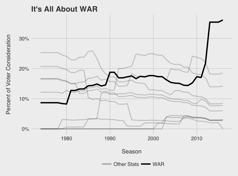
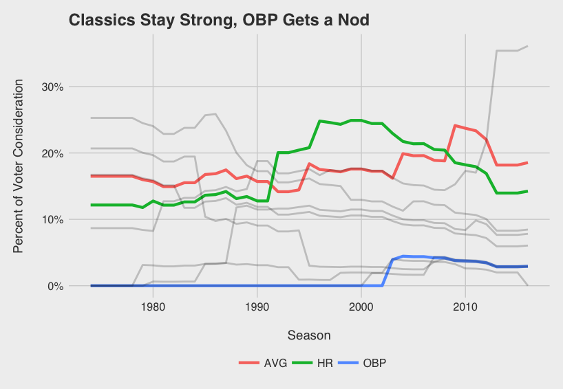
Visualizing the way Jarvis considers different factors (i.e. how the model’s weights change) over time for position players reveals trends in voter behavior.
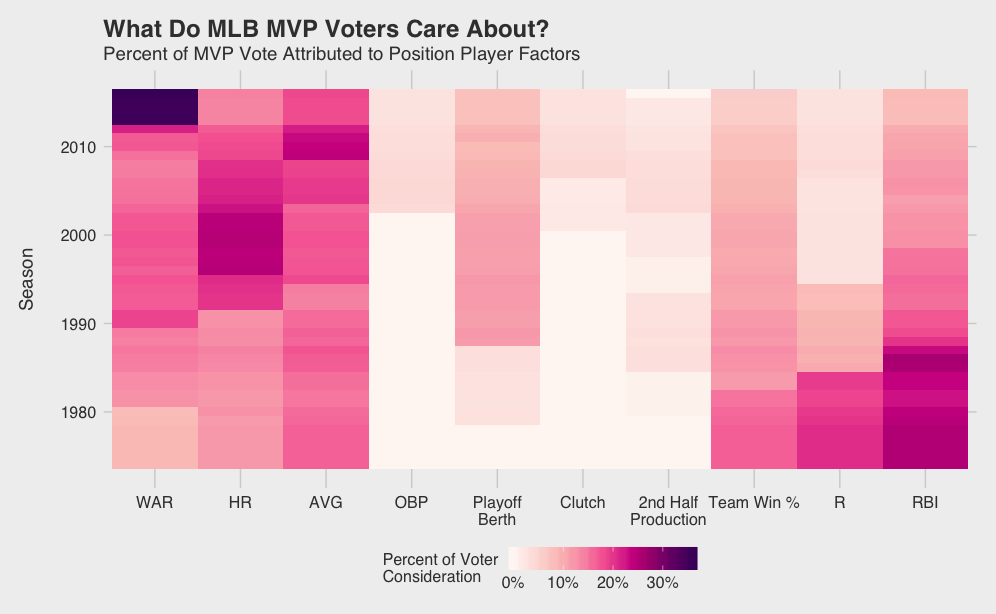
Immediately obvious is the recent dominance of WAR. As WAR becomes socialized and accepted, it seems voters are increasingly factoring WAR into their voting decisions. What I’ll call the WAR era started in 2013 with Andrew McCutchen leading the Pirates to their first winning season since the early 90’s. He dominated Paul Goldschmidt in the NL race despite having 15 fewer bombs, 41 fewer RBIs, and a lower SLG and OPS. While Trout got snubbed once or twice since 2013, depending on how you see it, his monstrous WAR totals in ‘14 and ‘16 were not overlooked.
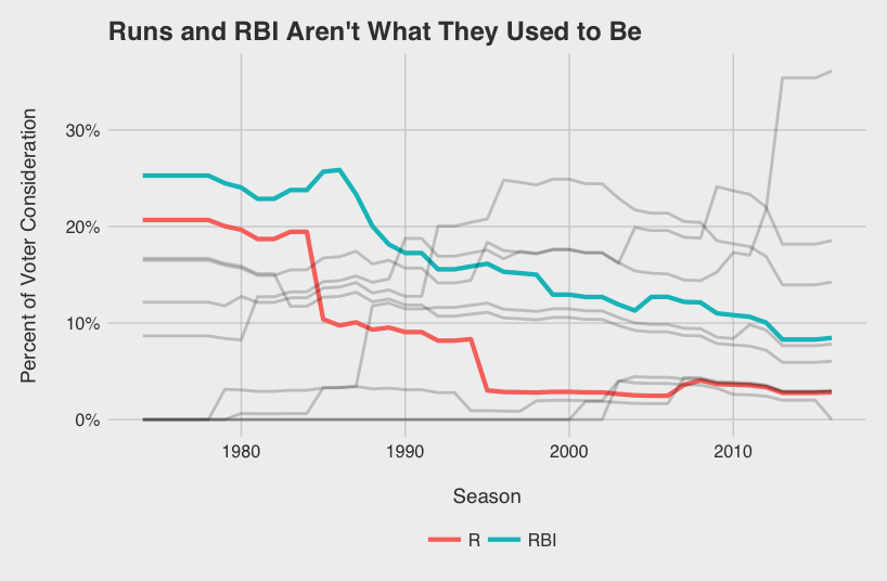
As voters have recognized the value of WAR, they have slowly discounted R and RBI acknowledging the somewhat circumstantial nature of the two stats. The “No Context” era from ‘74 to ‘88 can be characterized perfectly by the 1985 AL MVP vote. George Brett (8.3 WAR5), Rickey Henderson (9.8), and Wade Boggs (9.0), were all beat out by Don Mattingly (6.3) likely because of his gaudy 145 RBI total.
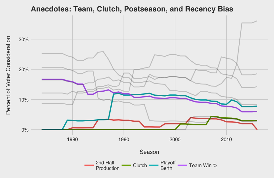
Per the voting rules, winners don’t need to come from playoff bound teams, yet this topic always surfaces during the MVP discussion. Postseason certainly factored in when Miggy beat out Mike Trout two years in a row starting in 2012. See that playoff berth bump in 2012 on the graph below? Yeah, that’s Mike Trout. What the model doesn’t consider, however, are the storylines, the character, pre-season expectations: all the details that are difficult for a bot to quantify. For example, I’ve seen a couple of arguments for Paul Goldschmidt as the frontrunner to win NL MVP after leading a Diamondbacks team with low expectations to the playoffs. I’ll admit, sometimes the storylines matter, and in a year with such a close NL MVP race, it could push any one player to the top.
What can I say about AVG and HR? AVG is a useless stat by itself when it comes to assessing player value, but it’s engrained in everyone’s mind. It’s the one stat everyone knows. Hasn’t everyone used the analogy about batting .300 at least once? Home runs\dotsthey are sexy. Lets leave it at that. Seems like these are always on the minds of MVP voters and are not likely to change any time soon.
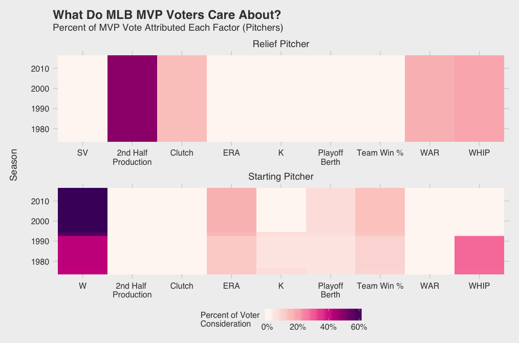
I’m sure some of you are already thinking, “What about pitchers!?” Don’t worry, I haven’t forgotten — although it seems MVP voters have. Only 3 SP and 3 RP have won the MVP award since 1974, and only about 7.5% of all top 5 finishers. As you can see in the factor weight graph below, their sparsity in the historical data results in little influence on the model; voters opinions don’t change often and their raw weights tend to be lower than position players. Overall, it seems as though wins continue to dominate the SP discussion along with ERA and team success. While I would expect saves to have some influence, voters tend to be swayed by recency bias and clutch performance along with WHIP and WAR.
What would an MVP article be without a prediction? Using the model geared to predict the winners, here are your 2017 MLB MVPs:
AL MVP: Jose Altuve Runner Up: Aaron Judge
NL MVP: Joey Votto Runner Up: Charlie Blackmon
Here are the results from the model tuned to return the best top 3 and top 5 finisher order:
| Rank | AL MVP | NL MVP |
|---|---|---|
| 1 | Jose Altuve | Charlie Blackmon |
| 2 | Aaron Judge | Nolan Arenado |
| 3 | Jose Ramirez | Giancarlo Stanton |
| 4 | Mike Trout | Joey Votto |
| 5 | Corey Kluber | Clayton Kershaw |
It’s apparent that I adjusted rate and counting stats for league and not park effects given both Rockies6 place in the top 2. Certainly, if voters are sensitive to park effects, Stanton and Turner get big bumps and Rockies players likely don’t have a chance. Larry Walker was the only Colorado player to win the MVP since their inception in 1993, but in a close 2017 race it might make the difference.
Continue reading below for the complete methodology and checkout the code on github.
Statistical Adjustments
Note: lgStat = league (AL/NL) average for that stat, qStat = league average for qualified players, none of the adjusted stats are park adjusted
There were two different adjustments needed for position player rate stats and count stats.
Rate stat adjustment: AVG+ = AVG/lgAVG
Count stats: HR, R, RBI
Count stat adjustment: HR Above Average = PA*(HR/PA - lgHR/PA)
There were three different adjustments needed for starting pitcher (SP) and relief pitcher (RP) rate stats and count stats.
Rate stats: ERA, WHIP
Rate stat adjustment: ERA+ = ERA/lgERA
Count stats I: K
Count stat I adjustment: K Above Average = IP*(K/IP - lgK/IP)
Count stats II: Wins (W), Saves (SV)
Count stat II adjustment: Wins Above Average = GS*(W/GS - qW/GS)
Fused Lasso Linear Program
I combined two different approaches to create a model I thought would work best for the purpose of predicting winners and illustrating change in voter opinions over time. Stephen Ockerman and Matthew Nabity’s approach to predicting Cy Young winners was the inspiration for my framework for scoring and ordering players. A players score is the dot product of the weights (consideration by the voters) and the player’s stats.
Note: On a mobile device turn sideways to see full formulas
\[ \text{Seasons:} \; Y = \{ 1974 \dots 2016 \} \] \[\text{Leagues:} \; L = \{ AL, NL \} \] \[\text{Ranks:} \; R = \{ 1 \dots \min{\{10, \text{players receiving votes}}\} \} \\ \text{Note: } \: R \setminus max = \{r \in R | r \; \neq \; \max{R} \}\] \[\text{Statistics:} \; S = \{ \text{All position and pitcher statistics} \} \] \[x_{ylrs} \; = \; \text{stat value in season y, league l, player with rank r of R, and statistic s}\] \[w_{ys} \; = \; \text{weight values on statistic s in season y}\] \[ \sum_{s \in S} w_{ys}x_{ylrs} \;\;\; \text{(rank r player score in season y and league l)}\]The constraints in the optimization require the scores of the first place player to be higher than the second place, and so on and so on. This approach, however, doesn’t allow for violation of constraints. I add an error term for violation of these constraints, and minimize the amount by which they are violated.
\[e_{ylr} \; = \; \text{violation of ranking constraints between player rank r and rank r+1}\] \[\min_{w} \sum_{y \in Y}\sum_{l \in L}\sum_{r \in R \setminus max } e_{ylr}\] \[\text{subject to } \sum_{y \in Y} w_{ys}x_{ylrs} - w_{ys}x_{ylr+1s} + e_{ylr} \geq \epsilon, \; \forall y \in Y, l \in L,r \in R \setminus max\] \[ e_{ylr} \geq 0, \; \forall y \in Y, l \in L,r \in R \setminus max\]Instead of constraining the weights to sum to 1, I applied concepts from Robert Tibshirani’s fused lasso which simultaneously apply shrinkage penalties to the absolute value of weights themselves as well as the difference between weights for the same stat in consecutive years. This accomplishes two things: 1) it helps perform variable selection on statistics within years helping combat collinearity between some performance statistics, and 2) it ensures that weights don’t change too quickly overreacting to a single vote in one year.
\[\min_{w} \sum_{y \in Y}\sum_{l \in L}\sum_{r \in R \setminus max } e_{ylr} \; + \; \lambda_1\sum_{y \in Y}\sum_{s \in S} |w_{ys}| \; + \; \lambda_2\sum_{ y \in Y \setminus \{ 2016\} }\sum_{s \in S} |w_{y+1,s}-w_{ys}|\] \[\text{subject to } \sum_{y \in Y} w_{ys}x_{ylrs} - w_{ys}x_{ylr+1s} + e_{ylr} \geq \epsilon, \; \forall y \in Y, l \in L,r \in R \setminus max\] \[ e_{ylr} \geq 0, \; \forall y \in Y, l \in L,r \in R \setminus max\]However, this approach and formulation cannot be solved by traditional linear optimization methods since absolute value functions are non-linear. The optimization can be reformulated as follows:
\[\min_{w} \sum_{y \in Y}\sum_{l \in L}\sum_{r \in R \setminus max} e_{ylr} \; + \; \lambda_1\sum_{y \in Y}\sum_{s \in S} \alpha_{ys} \; + \; \lambda_2\sum_{y \in Y \setminus \{ 2016\}}\sum_{s \in S} \beta_{ys}\] \[\text{subject to } \sum_{s \in S} w_{ys}x_{ylrs} - w_{ys}x_{ylr+1s} + e_{ylr} \geq \epsilon, \; \forall y \in Y, l \in L,r \in R \setminus max\] \[w_{ys} \leq \alpha_{ys}, \; \forall y \in Y, s \in S\] \[-w_{ys} \leq \alpha_{ys}, \; \forall y \in Y, s \in S\] \[ w_{y+1,s}-w_{ys} \leq \beta_{ys}, \; \forall y \in Y \setminus \{2016\} , s \in S\] \[-w_{y+1,s}+w_{ys} \leq \beta_{ys}, \; \forall y \in Y \setminus \{2016\} , s \in S\] \[ e_{ylr} \geq 0, \; \forall y \in Y, l \in L,r \in R \setminus max\]To select the lambda parameters, I trained the model using the first 10 seasons of scaled data7 increasing the training set by 1 season each time and tested with the subsequent year’s vote.
References:
1. Ockerman, Stephen and Nabity, Matthew (2014) “Predicting the Cy Young Award Winner,” PURE Insights: Vol. 3, Article 9.
2. R. Tibshirani, M. Saunders, S. Rosset, J. Zhu, and K. Knight. Sparsity and smoothness via the fused lasso. Journal of the Royal Statistical Society Series B, 67(1):91–108, 2005.
-
Predicts winners with 62.1% accuracy. ↩
-
On average predicts player positions 1.6 positions off in the top 5. For example, if a player is 3rd in votes but is predicted to place 5th, the player would be 2 positions off. ↩
-
First year FanGraphs provided specific data splits I needed. ↩
-
All player level data is from FanGraphs. ↩
-
Remember this is an average of FG and BRef ↩
-
Coors Field’s mile high thin air tends to increase offensive production. ↩
-
After in season statistical adjustments, I scaled the stats by mean and standard deviation of training data to enable comparison across coefficients. All position player stats were replaced with 0 for pitchers and vice versa. ↩