- Introduction
- Temporal Point Processes
- Injury Data
- Interpreting the Parameters
- Performance
- Mike Trout
- References & Resources
- Footnotes
Introduction
Anyone can admit that baseball is hard to predict1, probably one of the reasons it can be so exciting. I’ve definitely done my share of modeling game and at-bat outcomes, but I wanted to pose a different challenge for this post: predicting injury risk.
Injury risk is an important element of season long unpredictability. A bunch of injury research focuses mostly on pitcher health, looking at pitch load, movement, even video analysis. I’m sure teams also have their own complex systems for modeling and monitoring player health.
I’m going to keep the inputs (relatively) simple and limit the problem to predicting future injuries using only past injuries. Yes, it makes this problem a bit harder by not having any in-game information such as pitch load or changes in pitch/exit velocity. However, a certain statistical concept is well suited to clearly illustrate and quantify how injury history influences future injury risk: the self-exciting point process (SEPP) or Hawkes process (HP).
Using a HP we can answer questions like: Are injuries to specific body parts self-exciting – for example, do elbow injuries increase the likelihood of elbow injuries much more than other body parts? Does this differ in pitchers vs batters? How do day-to-day injuries influence future injury risk? Do past injuries increase future risk to related parts of the body? How do we put this information together to gauge injury risk at any point in time?
Temporal Point Processes
To understand how HPs can help to answer this I’ll first give some background on temporal point processes and how we might be able to use them. If you are familiar or just want to skip the math, go here.
A temporal point process (TPP) is a random process that results in discrete event occurrences over time. We can think about and define TPPs in a couple of ways
- A counting process - define a probability distribution over the number of events in an interval
- Intervals or interarrival times - define a probability distribution of the interval of time between successive events
Poisson Point Process
The most commonly known manifestation is the Poisson point process. The counting process is fittingly parameterized by a poisson distribution. Formally, the number of events $N(t)$ in an interval of time $t$ is a poisson distribution with mean $\lambda t$, where $\lambda>0$ is the rate or intensity of events on average in the interval. Remembering the formula for a poisson distribution, we can write the probability of a specific number of events $k$ occurring as:
\[P(N(t)=k) = \frac{e^{-\lambda t}(\lambda t )^k}{k!}\]To reframe this process around interarrival times, we can look at the probability of no events occurring in the interval $P(N(t)=0)$ or, in other words, probability of the next event occuring after $t$, $P(X>t)$.
\[\begin{align} P(N(t)=0) = P(X>t) & = \frac{e^{-\lambda t}(\lambda t )^0}{0!} \\ P(X>t) & = e^{-\lambda t} \\ P(X\leq t) & = 1 - e^{-\lambda t} \end{align}\]The last line is actually the same as the cumulative distribution for the exponential distribution with mean $\frac{1}{\lambda}$ and density $f(t) = \lambda e^{-\lambda t}$. So therefore, a poisson point process with rate $\lambda$ can also be modeled as events with random interarrival times according to an exponential distribution with an average time of $\frac{1}{\lambda}$.
The poisson process inherits a useful “memoryless” property from exponentially distributed arrival times which says that the probability of waiting X more minutes for a new event is independent of the past. This property shows up in the real world commonly in customer arrival settings (customers visiting a website, customers arriving at a store, etc), scoring goals in a soccer game, or the time it takes until your next car accident.
Homogeneous vs Nonhomogeneous
Often though, the real world is more complex than these simplifying assumptions. Usually, we don’t deal with rates or intensities that are truly constant as in the traditional homogeneous poisson process.
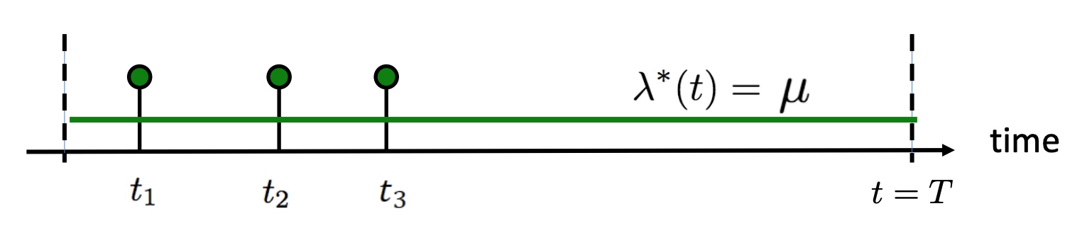
Homogeneous poisson process has an intensity $\lambda(t)$ which is always constant (Rodriguez & Valera, 2018).
Intensity is often a continuous function and fluctuates with time as modeled by an inhomogeneous poisson process. For example, customers’ rate of arriving at a store probably depends on the time of day as well as the day of the week.
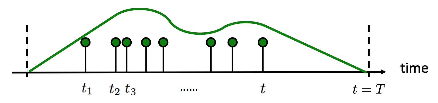
Inhomogeneous poisson process has an intensity $\lambda(t)$ which varies over time (Rodriguez & Valera, 2018).
Self-Exciting Temporal Point Process
We can generalize the concept of TPPs even further. While inhomogeneous poisson processes can vary their intensity over time, the number of events that occur in non-overlapping time intervals are still independent of each other. In other words, no matter how many events occur from $t_1$ to $t_2$, it shouldn’t change our expectation of the number of events from $t_2$ to $t_3$.
A Hawkes Process breaks these properties by using an intensity that is determined by previous events, or its history $\mathcal{H}_t$. There are many different ways we can link past events to the likelihood of future events, but the HP is specifically self-exciting which implies that the closer we are to past events the more likely we are to see a new event occur. In math terms it looks like
\[\begin{align} \lambda(t | \mathcal{H}_t) & = \mu + \alpha \sum_{t_i<t} \phi(t-t_i) \\ & = \mu + \alpha \sum_{t_i<t} e^{-\delta(t-t_i)} \end{align}\]where $\mu$ is some baseline or average rate of events, $\alpha$ is the degree to which a past event excites a new event, and $\phi$ is a kernel that basically tells us how much past events’ influence changes over time. An exponential kernel is commonly used in HP modeling, and assumes that past events’ influence decays exponentially over time.
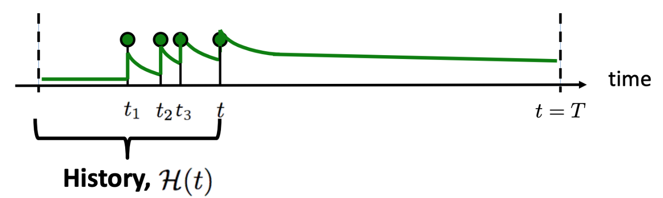
Self exciting point process where the intensity of events depends on the process history. (Rodriguez & Valera, 2018).
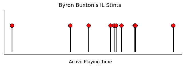
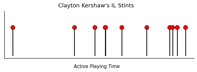
This type of process and its assumptions can lead to clustering of events as they feed off of each other’s excitement and the intensity at time $t$ rises. We can sometimes see this behavior where injuries compound and cluster together. Buxton and Kershaw’s injury timelines, for example, have similar short periods of successive injuries.
Modeling Multiple Event Types
Now we just need a few things in order to extend these models to injury prediction. First, we need a multidimensional framework for multiple event types. An overall intensity can be split into $K$ different intensities for each event type.
\[\begin{align} \lambda(t | \mathcal{H}_t) & = \sum_k \lambda_k(t | \mathcal{H}_t) \end{align}\]For any event type $k$, the intensity $\lambda_k(t)$ can be influenced by itself any other event $j$ through $\alpha_{j,k}$ and can decay at a different rate $\delta_{j,k}$.
\[\begin{align} \lambda_k(t | \mathcal{H}_t) = \mu_k + \sum_{j =1}^K\sum_{t_i<t} \alpha_{j,k} e^{-\delta_{j,k}(t-t_i)} \end{align}\]Finally, we need a way to learn the parameters of our model. After a lengthy derivation2, which I will skip, we can utilize the log-likelihood over a time interval $[0, T]$:
\[\mathcal{L} = \sum_{i:t_i < T} \lambda_{k_i}(t_i) - \int_0^T \lambda(t) dt\]In the first term, for each event occurrence $i$, we try to maximize the intensity for that event type $k_i$ at the time it occurred $t_i$. At the same time, in the second term, we minimize $\lambda(t)$ across the whole interval at all other points in time where no events occur. Though we can work out the full likelihood function, I just use gradient descent to optimize this function. To estimate the second term, we can sample points in the interval $[0, T]$ and minimize the sum $\sum_s \lambda(t_s) \; \forall s \in samples$ .
For each injury, we only need the type $k$ and time $t$ to get started. This ends the math portion, onto the data!
Injury Data
In order to leverage a TPP to make inferences on injury risk, I needed to source IL, day-to-day (DTD), and player game data. Luckily, MLB stats api provides IL stint data and Pro Sports Transactions logs MLB DTD data ( I initially got the idea to work with injury data from Derek Rhoads’ injury dashboards and would like to thank him for pointing me to Pro Sports! ). Finally, I compiled the dates of player games from my statcast database scraped from Baseball Savant.
Cleaning all of the injury data was enough for a project in itself. I only concentrated on injuries during players’ time in the majors, so while we might not have a complete picture of player injury history, these resources together are sufficient given we make some simplifying assumptions:
- I use only injuries that occur during major league playing time
- The time between injuries is measured in active playing time - I assume that any time recovering or playing in the minors is not time that could result in “major league injuries”. The time span from an IL date to the next MLB game played I call an injury span and are excluded from the time between injuries.
- I exclude all injuries that are unlikely to be baseball related (e.g, sickness, infections, covid, etc. )
Additionally, I created categories for each injury by location, type, and IL/DTD. Each categorization is subjective, but I tried to keep them as specific as possible without having lopsided distributions. On occasion, players will have multiple injuries during an injury span, in which case I take the injury with the longer IL stint 3.
For more details on how the data is scraped or processed, you can check out the code on github.
Interpreting the Parameters
We can train models with any kind of event encoding. For example, we could use any combination of the location, type, severity, or length of the injury to come up with categories to predict. The more categories we use, the more sparse the data. For simplicity, I trained models using the location of the injury and optionally if it resulted in an IL stint or just day-to-day (DTD) status.
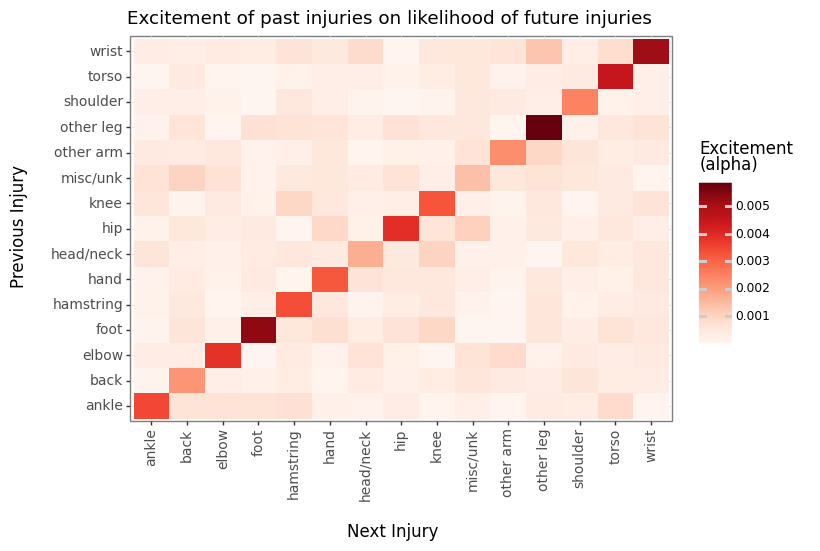
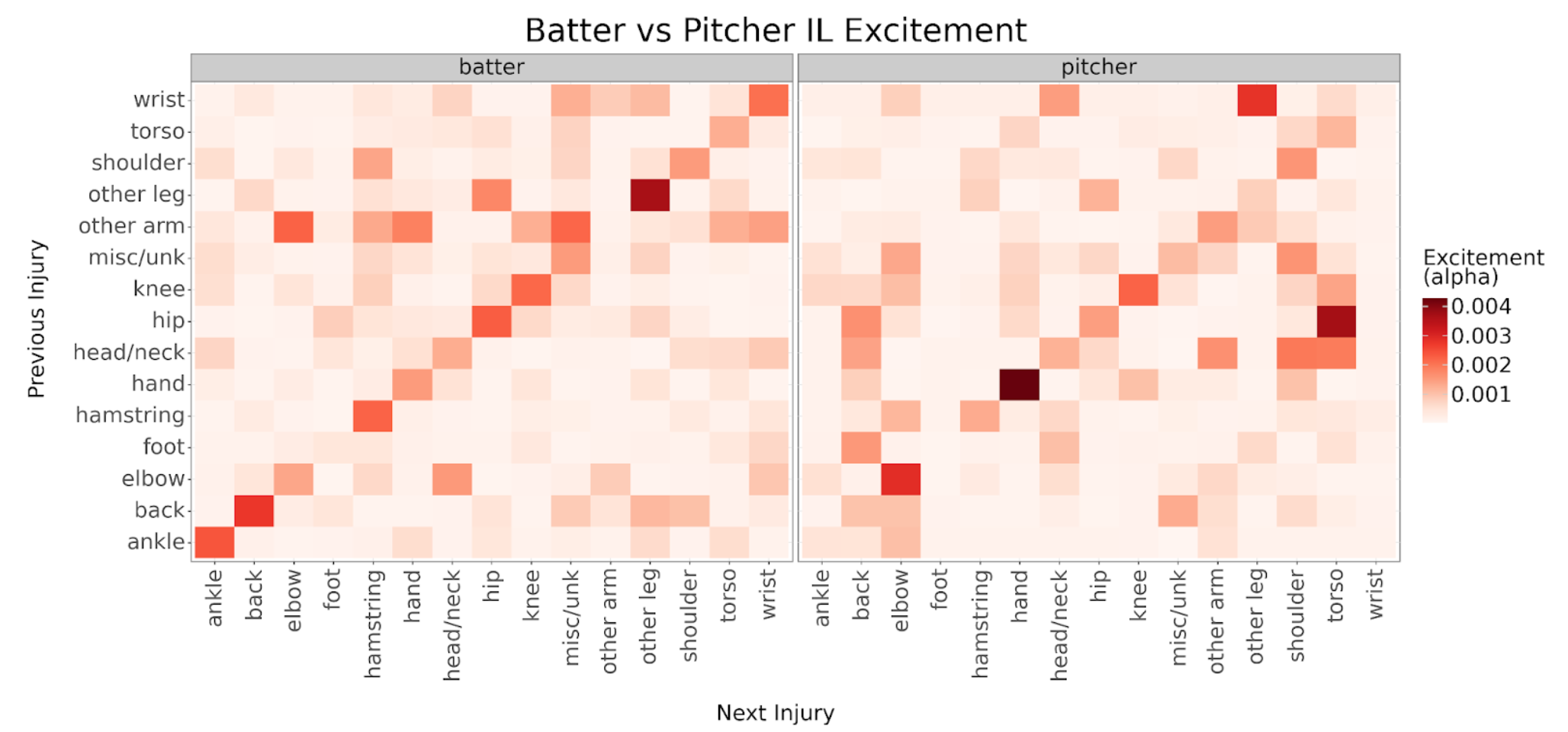
First, by inspecting the excitement (alpha) matrices of the location only model, we can see a really clear self-excitement trend. Previous injuries tend to drastically increase the intensity of injuries in the same location.
If we break down the model into separate events for IL and DTD injuries, we see that DTD injuries tend to drive a lot of the self-excitement.
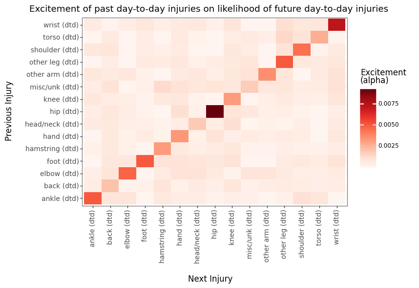
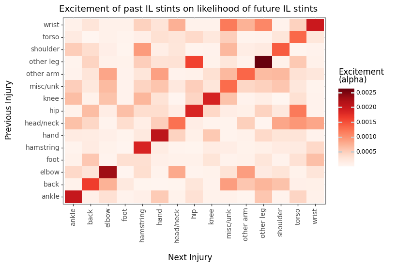
IL stint self-excitement is a bit more muted relative to other alphas. Generally, this makes sense since IL stints can range from 10 days to a whole season for a surgery meaning there can be a large variance in the amount of recovery and therefore future injury risk. DTD injuries are probably more correlated with nagging problems that might end in an IL stint where layers might be day to day with that same injury multiple times.
We can see some large excitement off the diagonal that adhere to intuition such as hip, head/neck injuries preceding torso issues or elbow and wrist injuries preceding other arm injuries. Though there are a handful of others that may be more confusing and likely coincidental, like wrist injuries preceding other leg injuries.
We can dig even deeper by building separate models for batters and pitchers. These breakdowns can illustrate differences in batter and pitcher injury excitement. For example, hip and head/neck injuries have a larger effect on future torso and shoulder injuries for pitchers while higher alphas on the diagonal suggest batters tend to aggravate their ankles, backs, legs, and wrists more often.
We can also leverage information from the decay kernel for more insights on how injuries raise future injury risk. In the plot below we can see how pitchers’ injuries lead to varying future elbow injury risk.
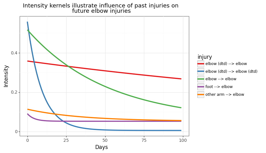
The blue line illustrates the high self-excitement of DTD injuries, initially having a very high risk, but decaying quickly. DTD elbow and IL elbow injuries have the longest persistent effect on future elbow related IL risk (red and green line respectively). Other arm injuries have little effect and risk of elbow IL stints immediately revert to the long term average after a foot injury.
Performance
TPPs are interpretable and good estimators of risk over time, given the data adhere to our assumptions. We can predict outcomes in many ways using TPPs:
- Given the time of the next injury, what injury do we expect?
- Over a time range, what is the most likely injury?
- What is the expected time of the next injury?
To generate predictions, I use a two step process: I first estimate the time of the next injury, and given that time I predict the injury location.
The injury distribution is fairly balanced. The model should be able to surpass a 10% accuracy naive baseline predicting hamstring injuries every time.
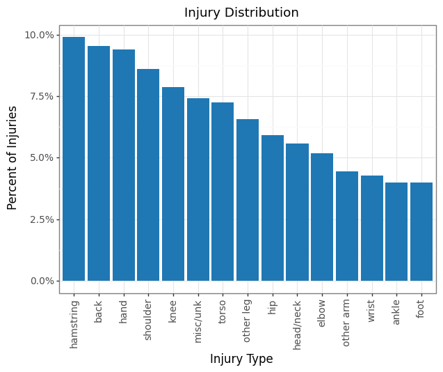
The TPP model predicts the injury correctly 18.5% of the time out of the 15 different categories. The correct injury also falls in the top 2 and top 3 predictions 30% and 37% of the time respectively. The TPP IL/DTD model (broken down into IL/DTD) recalls the actual injury 14% of time with double the possible categories.
I am able to reduce the large uncertainty in the timing of injuries as well from 162 day RMSE using a naive average time between injuries to 144 days using a TPP.
| Metric | TPP | TPP IL/DTD |
|---|---|---|
| # of Categories | 15 | 30 |
| Top Category Prevalence | 10% | 7% |
| Model Top 1 Acc | 18.5% | 13.8% |
| Model Top 2 Acc | 30.2% | 21.1% |
| Model Top 3 Acc | 36.8% | 27.9% |
| Time RMSE (days) | 144.3 | 144.1 |
Mike Trout
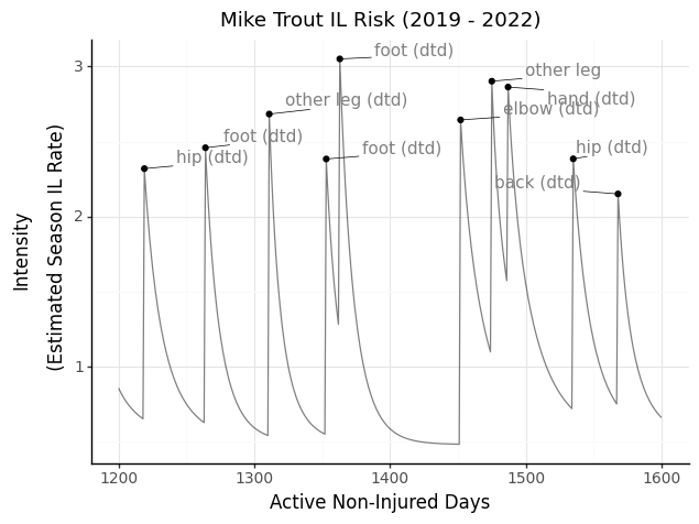
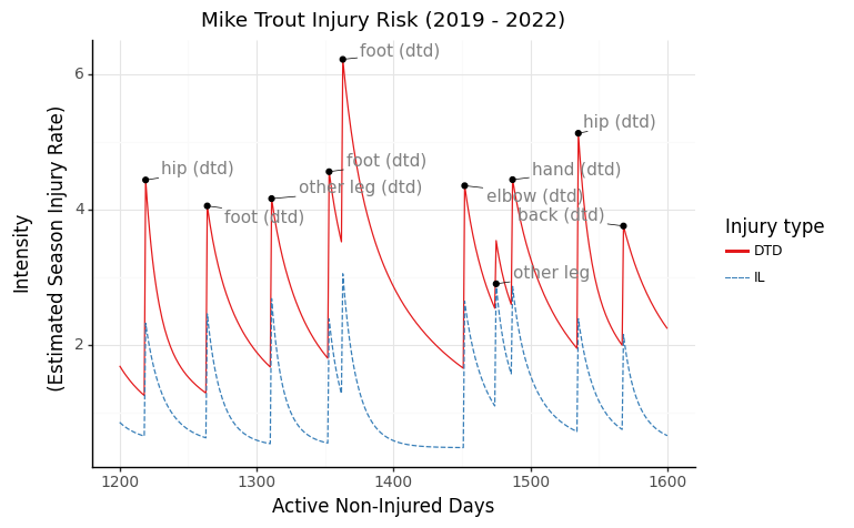
To get a sense of how we can illustrate individual players with TPPs, I looked at the last few years of Mike Trout’s injury history. First, we can view Trout through the lens of overall IL risk during his in-season non-injured days, where each labeled point is one of his injuries. The intensity is modeled in terms of an instantaneous daily rate, so when scaled by 180 days, approximates the season-long IL rate.
We can also view DTD and IL risk side by side.
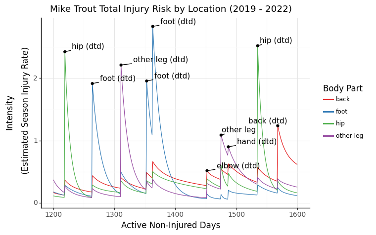
Finally, the most interesting way to view injury risk: broken down by location. We can really see how different injuries cause changes in the intensities of other body parts. For example, Trout’s calf injury in mid-2019 (approx day 1300) elevated his risk of foot injuries, possibly foreshadowing his foot issues later in the year.
TPPs are useful tools for learnable processes that evolve over time. Though I have a tendency to overuse baseball data (sorry not sorry), TPPs are more popular in social media, e-commerce, and recommendation applications. TPPs continue to evolve and progress, most recently being parameterized with neural networks (LSTM, Transformer) making them much more powerful and flexible.
For more details, check out the code on github.
Data Sources: Baseball Savant, Pro Sports, MLB Stats API
Photo Credit: Mark Brown / Getty
References & Resources
-
Rodriguez, Manuel and Valera, Isabel. 2018. Learning with Point Processes (ICML 2018 Tutorial): Part 1,2,3
-
Rizoiu et al. 2017. A tutorial on Hawkes Processes for events in social media. https://arxiv.org/abs/1708.06401.
-
Mei, Hongyuan and Eisner, Jason. 2017. The Neural Hawkes Process: A Neurally Self-Modulating Multivariate Point Process. https://arxiv.org/abs/1612.09328.
Footnotes
-
How often does the best team win? A unified approach to understanding randomness in north american sport. ↩
-
Log-likelihood derivation in Appendix B ↩
-
If there are any miscellaneous injuries, I take one of the non-misc injuries in the span. If there are ties in IL time, I break ties with a priority order of injuries. ↩